How to Make a 2D Physics Engine (Collider + Rigidbody)

Welcome. In this post, I’ll be describing my implementation of the collider and rigidbody classes. If these terms are unfamiliar, I recommend you take a quick look at my previous post, where I provide an overview of the various components of a physics engine. To summarise: a rigidbody stores the physics properties of the GameObject, while the collider stores its shape and material properties. Although (or perhaps because) these two classes form the core of any physics engine, they are comparatively straightforward and generic.

All of the code is written in Python, and is taken from my physics engine implementation on Github. In turn, these files were essentially transcribed from my original project in Rust, which is still incomplete (I ended up sticking with the Python rendition).

rigidbody.py

class Rigidbody():
    def __init__(self, mass, inertia, position, angle=0):
        self.inv_m = 0 if mass == 0 else 1. / mass
        self.inv_i = 0 if inertia == 0 else 1. / inertia

        self.p = position
        self.v = np.zeros(2)
        self.f = np.zeros(2)
        
        self.a = angle
        self.w = 0.
        self.t = 0.

        self.R = np.zeros((2, 2))
        self.updateR()

        self.awake = True
    
    def updateR(self):
        c, s = np.cos(self.a), np.sin(self.a)
        self.R[0, 0] = self.R[1, 1] = c
        self.R[1, 0] = s
        self.R[0, 1] = -s

    def add_force(self, force, at):
        self.f += force
        self.t += np.cross(at - self.p, force) 

    def add_impulse(self, impulse, at):
        self.v += self.inv_m * impulse
        self.w += self.inv_i * np.cross(at - self.p, impulse)

    def update(self, dt):       
        self.v += self.f * self.inv_m * dt
        self.p += self.v * dt
        self.f = np.zeros(2)
 
        self.w += self.t * self.inv_i * dt
        self.a += self.w * dt
        self.t = 0.

        self.updateR()
    
    def l2g(self, v, vec=False):
        return v @ self.R if vec else v @ self.R + self.p
    
    def g2l(self, v, vec=False):
        return v @ self.R.T if vec else (v - self.p) @ self.R.T

Some comments:

• It’s easier to directly store the inverse of mass or inertia, since we then have to avoid computing $1/ m$ at each timestep. Divisions are expensive!

• In 2D, all angular variables are scalars. In 3D, angular variables are also 3D, but this is more a coincidence than anything; this relation does not hold in any other dimension

• We store both the scalar angle as well as the orientation matrix \(\begin{pmatrix}\cos\theta&\sin\theta\\-\sin\theta&\cos\theta\end{pmatrix}\) which is much more useful to convert vectors and points from global to local frame and vice versa. We must make the distinction between vectors and points here, since vectors are only defined by the difference between two points and so need not be translated between frames.

• Methods are provided to update both force and impulses. This is foreshadowing: for reasons of stability and accuracy, the physics engine will work directly at the level of impulses while resolving constraints. These also add in torque and angular velocity respectively, which are constructed through the cross product: $\tau_\text{2D}=\lVert\vec r\times\vec F\rVert$.

• The velocity and position (and their angular counterparts) are then updated by the discrete versions of the equations $\Delta \vec v=\int\mathrm dt\ \vec a\Rightarrow\Delta \vec v=m^{-1}\vec F\Delta t$. $\Delta t$ is determined by the frame rate and supplied by the engine in order to keep the updates smooth. Importantly, velocity is updated before the position, so the position update employs the new velocity. This is the Semi-implicit Euler method of integration, and surprisingly yields a lower error than if we were to integrate them in the reverse order.

• Inertia is much easier to implement in 2D than in 3D, where inertia becomes a whole tensor and has to be updated based on the orientation matrix (which, incidentally, requires renormalisation, often using quaternions)

collider.py

class AABB():
    def __init__(self, min_, max_):
        self.min, self.max = min_, max_
    
    def intersects(self, other):
        return ((self.min <= other.max) & (self.max >= other.min)).all()
    
    def glVerts(self):
        return (self.min[0], self.min[1], self.max[0], self.min[1],
             self.max[0], self.min[1], self.max[0], self.max[1],
             self.max[0], self.max[1], self.min[0], self.max[1],
             self.min[0], self.max[1], self.min[0], self.min[1])

class Collider():
    def __init__(self, verts, restitution=1.0, friction=.8, density=1.0, offset=np.zeros(2)):
        self.density = density
        self.area = 0
        self.centroid = np.zeros(2)
        
        vverts = np.zeros((verts.shape[0] + 1, verts.shape[1]))
        vverts[:-1], vverts[-1] = verts, verts[0]
        
        for i in range(vverts.shape[0] - 1):
            a = vverts[i, 0] * vverts[i + 1, 1] - vverts[i + 1, 0] * vverts[i, 1]
            self.area += a
            self.centroid += a * (vverts[i] + vverts[i + 1])
        
        self.area *= 0.5
        self.centroid /= 6 * self.area
        self.verts = verts - self.centroid + offset
        self.res = restitution  
        self.mu = friction
    
    def edges(self):
        edges = np.zeros_like(self.verts)
        edges[:-1] = self.verts[1:] - self.verts[:-1]
        edges[-1] = self.verts[0] - self.verts[-1]
        return edges

    def aabb(self):
        return AABB(np.min(self.verts, axis=0), np.max(self.verts, axis=0))

    @staticmethod
    def regular_polygon(n, size):
        verts = np.exp(np.arange(n) * np.pi * 2j / n) * size
        return Collider(verts.view('(2,)float'))
    
    @staticmethod
    def random_polygon(n, size):
        angles = np.cumsum(np.random.rand(n))
        angles = angles / np.max(angles)
        verts = np.exp(angles * np.pi * 2j) * size
        return Collider(verts.view('(2,)float'))

• First, the Collider class: it stores an ordered set of vertices and material properties such as the friction and restitution (“bounciness”). Using the shoelace formula and its derivatives, we can compute the centroid and area of the polygon, the latter of which can be multiplied with density to obtain the mass of the collider. However, since we envision objects with multiple colliders associated to them, an offset can also be supplied, which translates the centroid of the collider away from the true centre of the composite object.

• There are also straightforward methods for obtaining the edges of the collider and regular and random convex polygons. The latter algorithm is neat: random angles between $0$ and $2\pi$ are generated and then the points on a circle corresponding to these angles are sewn up.

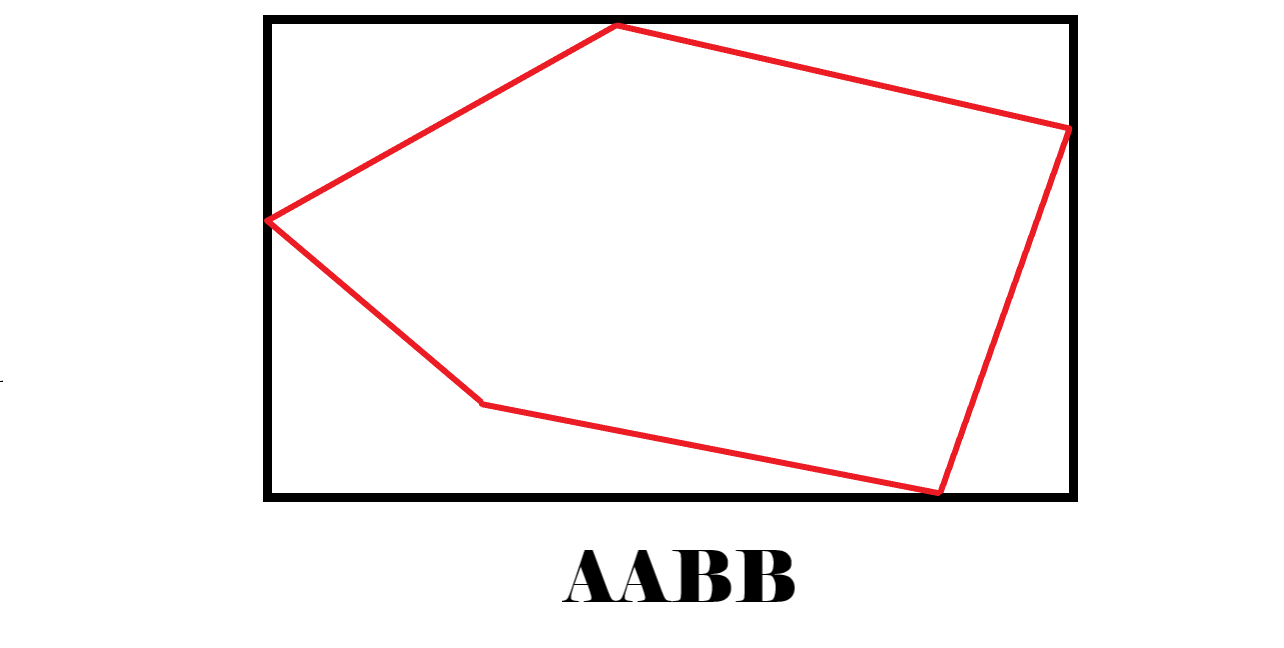
• Now for the AABB (axis-aligned bounding box) class. This is simply a non-rotated rectangle which encloses the polygon perfectly, and is specified by its bottom-left and top-right corner positions. This solely exists to improve collision detection speeds: rather than immediately jumping into an expensive collision detection routine for each pair of bodies, we can instead discard a sizeable portion of the pairs if their AABBs do not intersect (the intersection test for AABBs is extremely fast). After isolating those pairs which actually stand a chance of intersecting, we perform the full-fledged SAT-GJK routine to identify the true positives. Some people use oriented bounding boxes, where the bounding rectangle can be rotated. This leads to tighter fitting boxes and hence better pair pruning, at the expense of a more involved and time-consuming computation and intersection test.