Hi, I’m back again, returning after a somewhat extended hiatus from physics. For one thing I’ve been doing a lot of competitive programming practice (Leetcode, Codeforces, Google Code Jam Archives - dynamic programming is a favourite), which honestly deserves a whole post of its own. Back in the realm of physics, a lot of my current exploration is in computational phys/chem, something which I hadn’t looked into much until now. Here’s what I’ve been working on lately:
-
I was also revising solitons in low dimensions - kinks, monopoles, vortices - because I’m planning on making a numerical simulation of $\phi^4$ kink-antikink-meson scattering. Since it’s a non-linear boundary value problem, I’ll probably be using the shooting method, which is a nice callback to the Griffiths Chapter 2 exercise. Plus I want to acquaint myself with Atiyah and Hitchin’s work on soliton moduli spaces, visualise the Kosterlitz-Thouless transition, and explicitly construct some skyrmion solutions/rational maps (incidentally, DAMTP is a huge hotbed for soliton research). Zee was pretty helpful for the physical interpretations here. In fact, I found Zee also contains the only good exposition I’ve seen of the fractional quantum hall effect from a field theory standpoint.
-
Density Functional Theory. I’ve wanted to make a simple, functioning DFT program for at least a year, but didn’t have the time until now. Unlike my previous analytical, Gaussian orbital-based Hartree-Fock code for helium, I opted to use a lattice-based plane-wave basis for periodic systems, for reasons of simplicity and novelty. Among other things, pinning down the physics was my first practical use case of the Obsidian.md note-taking application. The code is still a work in progress, but I’ve managed to get the first significant module, a Poisson equation solver, up and running - with NumPy and matplotlib of course. Although I was planning on making it in C++ or Julia, NumPy/Python has the huge benefit of being able to prototype a robust first iteration quickly. A major difference from other projects I’ve done (think the chess engine, or the physics engine) is that a proper DFT simulation is quite hard to debug - realistic computations involve matrices with over 10000 rows and columns, so I essentially have to develop optimisations right from the beginning. Initially, finding useful resources was a huge struggle: the core theory behind DFT is actually very simple, but details on computational implementations were very scarce. I did find DFTK.jl through the JuliaCon presentations (seriously, check those out), but the source code is no Stockfish, it felt genuinely hard to read. The ultimate resource was actually the Cornell mini-course lectures here, even though the arguably most important video is missing from the series. Anyway, the next steps will probably be speeding up my Poisson solver to include more basis functions, then implementing a simple LDA functional and gradient descent solver. The ultimate goal will be to find some thermodynamic properties of a ion lattice ab initio.
-
BFSS matrix theory. This is the paragon of simplicity returning after a drudging trek through the complex: it turns out that M-theory in a particular background and reference frame is conjectured to be equivalent to a (relatively) simple supersymmetric quantum mechanics system describing D0-branes in 10 dimensions, which I find incredible. I’m using https://arxiv.org/abs/0101126 as a “big picture” review and https://arxiv.org/abs/1708.00734 as an in-depth source. Hopefully I’ll be able to delve into the meat of the conjecture without getting bogged down in the endless pushing around of numbers that seems to be prevalent in supergravity computations. For fun I’m also revisiting quantum 3D gravity (first exposure around a year ago).
-
And joining the ranks of “learning the theory behind the numerical techniques without coding them” are Monte-Carlo methods for QFT, and lattice gauge theory. The day I actually implement these is the day my personal supercomputer cluster arrives.
Representing the Board State
Before commencing with an algorithm, we need to settle on our data structures - in particular, how do we represent the state of the chess board? An obvious method, particularly if you’re an OOP fiend, would be to use an array of Piece objects, with each piece type (knight, bishop, etc.) a class inheriting from Piece. If that’s what you thought of, discard it immediately! For extremely time-sensitive applications, you’ll find that these abstractions aren’t so zero-cost after all, and that working as close to the metal as possible is an advantage that you should seize with reckless abandon.
In particular, did you notice something familiar about the number of squares, 64? Yep, the largest integer type is stored in 64 bits, and can be efficiently manipulated by modern 64-bit processors. That’s why the fundamental object in fast chess engines is the bitboard. It’s a 64-bit integer with each set bit representing occupancy in the corresponding square. For instance, the integer 16 when written in binary representation is 1000, and 129 is 1000001. To see how this corresponds to a chess board, pad the number with 0s at the front, then put the 8 lowest bits from left to right in the lowermost row, the next 8 lowest bits in the row above it, and so on. Here’s what that looks like for the two examples I gave you:
0 0 0 0 0 0 0 0 | 0 0 0 0 0 0 0 0
0 0 0 0 0 0 0 0 | 0 0 0 0 0 0 0 0
0 0 0 0 0 0 0 0 | 0 0 0 0 0 0 0 0
0 0 0 0 0 0 0 0 | 0 0 0 0 0 0 0 0
0 0 0 0 0 0 0 0 | 0 0 0 0 0 0 0 0
0 0 0 0 0 0 0 0 | 0 0 0 0 0 0 0 0
0 0 0 0 0 0 0 0 | 0 0 0 0 0 0 0 0
0 0 0 1 0 0 0 0 | 1 0 0 0 0 0 0 1

16                129
These bitboards respectively represent the starting position of the white queen, and the white rooks! So the state of a board can be represented by 12 bitboards (2 colors $\times$ 6 piece types), which we update as the players make moves.
The question is why does this provide a speedup? It’s because all the generation and verification of legal moves in a position, in accordance with the complex rules of chess, can be rapidly executed using the bitwise operators: AND, OR, XOR and bitshifts. OK, so how is that beneficial? The best way to find out is how it overcomes the downsides of our original idea: an array of Piece objects.
Suppose we want to measure the amount of area controlled by our pawns, as a rough measure of piece mobility during the evaluation stage. In the Piece-Array paradigm, this would involve looping over each square on the board, checking whether it’s a pawn, then finding the squares to the north-left and north-right (provided of course they don’t fall of the board). If this sounds tedious, that’s because it is.
Au contraire, the bitboard technique is incredibly fast. Using a dot for zero, suppose we have a white pawn bitboard like so:
. . . . . . . .
. . . . . . . .
. . . . . . . .
. . . 1 1 . . .
. . 1 . . . . .
. . . . . 1 . 1
1 1 . . . . . .
. . . . . . . .
If we ignore the A-file and shift the bitboard 7 bits to the right, we get
. . . . . . . .
. . . . . . . .
. . 1 1 . . . .
. 1 . . . . . .
. . . . 1 . 1 .
1 . . . . . . .
. . . . . . . .
. . . . . . . .
These are the squares attacked by pawns in the north-west direction! Moreover, we can ignore the H-file and shift 9 bits to the right, to get
. . . . . . . .
. . . . . . . .
. . . . 1 1 . .
. . . 1 . . . .
. . . . . . 1 .
. 1 1 . . . . .
. . . . . . . .
. . . . . . . .
If we OR these together, we get the bitboard of all squares attacked by all our pawns. To find the area covered, we have to count the number of 1s, i.e. perform a popcount, for which extremely fast dark magic routines like “De Bruijn sequences” exist. And we’re done. Don’t lose sight of the fact that these bitboards are just numbers! So this entire function would be coded by something like:
// get the white pawn bitboard
Bitboard pb = board.bitboards[WHITE + PAWN]


//							   (no A-file for NW attacks )          (no H-file for NE attacks)
int area_attacked = popcount( ((pb & 18374403900871474942) << 7) | ((pb & 9187201950435737471) << 9) )
Of course, these numbers would be categorised into lookup tables rather than hardcoded. What’s more, each bitwise operation is even cheaper than an addition. This creates the speedup we were promised, especially since bitboard methods find use in all three stages of a chess engine.
Bitboards do have a major downside though. With our new data model, it becomes expensive to query which piece occupies a given square. To counter this we use the best of both worlds, by storing both an array of bitboards, and an 64-array of pieces, often called a mailbox. The bitboard array is indexed by piece type, while the mailbox is indexed by board square, and we have to update both while making a move (this duplication is practically trivial).
This forms the core of the board class, although as we will see later it will be useful to store additional data for
- complying with e.g. the 50-move rule or threefold repetition
- storing special bitboards computerd during the move generation phase for reuse in the later phases
Representing Chess Moves
Apart from the board, it is integral to have an efficient representation of chess moves - selecting the best move in a position is, after all, the objective of a chess engine. Fundamentally, a move is a pair of start and end squares: we don’t even need the piece being moved since this can be inferred form the board data. Let’s try and store this in 16 bits. A square is represented by 6 bits ($2^6=64$), so with uint16_t move = (from_square << 6) | to_square, we still have 4 bits left over, which we’ll call “flags”.
Flags contain the remaining info necessary to specify “special” moves. These include captures, pawn promotions, double pawn push, castling and en passant. As luck would have it, there are 16 possible combinations which fit snugly in the top 4 bits. While performing a move on a board, these flags need to be queried since they might make updates to the board state (e.g. you can only castle once).
Flags have a secondary purpose in the search phase. Certain types of moves, such as promotion captures, are likelier to be overwhelmingly better than other moves in the position. So before searching through the game tree, we can sort the moves heuristically so that if we chance upon a winning move earlier on, we save time by avoiding the rest of the branches.
And that’s all, on to move generation! The posts are probably going to get a lot longer from here.
You’ve probably heard of superconductivity - isn’t it the phenomenon where a material has zero resistance, usually at very low temperatures? It sounds simple, but it actually requires the full force of quantum mechanics to describe it, and this is what Bardeen, Cooper and Schreiffer did in their Nobel-prize winning work, 60 years ago. In this two part series, I’ll aim to describe the physics behind superconductors, which will involve interesting detours into solid state physics, electrodynamics and quantum mechanics.
A recurring motif in condensed matter systems like superconductors is fundamental degrees of freedom (like electrons, photons, etc.) conspiring to form emergent phenomena when viewed at a slightly larger scale. These phemonena can be described as being initiated by objects with different properties to the original, fundamental ones, and these objects are called quasiparticles. An easy-to-visualise example is of an electron hole: imagine a lattice of atoms. This has room for electrons to live, but the absence of an electron in its designated spot creates a hole. As it turns out, we can ascribe particle-like properties to this hole, regarding it as a fundamental object in its own right. Indeed, this was Dirac’s original interpretation of the antiparticle solutions to his famous equation.
Wavefunctions and quantum particles
Superconductors also involve an emergent phenomenon, but I must first digress to introduce some key aspects of quantum mechanics. I will emphasise the conceptual features and aim to keep mathematical notation to a minimum. As you might be aware, quantum mechanical objects do not have a definite position. Rather, they are described by a wavefunction which is a function of space and time, denoted $\psi(\mathbf r, t)$. At a given time, $\psi(\mathbf r)$ specifies a complex number at each point in space such that the probability of finding the particle in some infinitesimal volume $\mathrm dV$ is $\lvert\psi(\mathbf r)\rvert^2\mathrm dV$, where $\lvert\cdot\rvert^2$ denotes the magnitude squared. As opposed to this probability, the value of the wavefunction is not itself measurable. So why bother working with $\psi$ and not just with $\lvert\psi\rvert^2$ directly? Because, similar to light waves, when multiple wavefunctions (for instance, corresponding to two electron beams passing through different slits) coalesce, the wavefunctions $\psi_1$ and $\psi_2$ themselves add constructively and destructively (and not the probabilities $\lvert\psi_1\rvert^2$ and $\lvert\psi_2\rvert^2$) . A similar thing happens with classical electromagnetic waves: the (classical) waves add as $A=A_1+A_2$ - their individual intensities on a screen, given by $\lvert A_1\rvert^2$ and $\lvert A_2\rvert^2$, do not add! This is the reason electrons display the same band-like pattern on a screen as light rays during the double-slit experiment. Finally (although we will not need it here), the way these spatial probabilities change over time is governed by the famous Schrödinger equation.
Now for deep reasons, there are two categories of fundamental particles, bosons and fermions. Qualitatively, the difference is that no two fermions can have the same quantum state, while as many bosons can pile up into a given quantum state as they’d like. If these sound familiar, it’s because they describe the Pauli exclusion principle and the Bose-Einstein condensate respectively. Famous fundamental fermions include the electron, neutrinos, and all 6 quarks while photons and gluons are fundamental bosons.
For the same deep reasons as above, a composite object containing an odd number of fermions is still fermionic, such as a proton, which contains two up quarks and a down quark and similarly for the neutron. Indeed, that the Pauli exclusion principle continues to act for the proton and neutron is responsible for the structure of almost all visible matter in the universe! However when an object is composed of an even number of fermions actually acts as a boson. Why doesn’t the Pauli exclusion principle fundamentally prevent this? See here.
The atomic lattice
If you’ve digested this, it’s time to move on to the superconductor setup. It’s not very difficult - we just need a lattice of metal atoms. Assume for now that the metal ions are fixed in place, and the electrons don’t interact with anything. As simple as it sounds, the finite-size lattice actually forces electrons to take on discrete values of momentum. In fact, this is not too hard to visualise: quantum mechanics tells us that particles have a wavefunction. The momentum of a wave is given by how rapidly it is changing, or in other words its frequency. But imagine (or try!) attaching a string, another wave-producing object, between two beams at a distance of $L$. If you pluck the string at different places, you’ll find that only certain wavelengths $\lambda_n$ persist after a few seconds. This is the case when $\lambda_n=\frac{2L}{n}$ - that is, wavelength can only take on a set of discrete values (or else the vibration dies out by destructive interference). Since frequency is just speed divided by wavelength, the possible frequencies form a discrete set: $f_n=\frac{vn}{2L}$. Analysing the Schrödinger equation for an electron in the finite, periodic lattice uses essentially the same argument to conclude that the electron’s momentum also takes on a set of discrete values. We say that momentum is quantized - but instead of $v$ in the previous formula, we have a factor of $2\pi\hbar$, where $\hbar$ is Planck’s constant, signalling the presence of quantum mechanics. So $p_n=\frac{n\pi\hbar}{L}$. We see that the larger the dimensions of the lattice are, the less spaced out the possible momenta. One more thing - our system has three finite dimensions, so the possible discrete momenta themselves form a 3-dimensional lattice, known as the reciprocal lattice. The sites of this lattice are the obvious generalisation of the one-dimensional case: $p=(p_x, p_y, p_z)$ are the three components of momentum in different directions. So for instance, $p_{1,0,0}=\left(\frac{\pi\hbar}{L}, 0, 0\right)$, $p_{0,1,0}=\left( 0,\frac{\pi\hbar}{L}, 0\right)$, $p_{43, 9, 17} = \left(\frac{43\pi\hbar}{L}, \frac{9\pi\hbar}{L}, \frac{17\pi\hbar}{L}\right)$, and so on. Hopefully you’ll be able to keep track of whether I’m talking about the physical metal lattice or the momentum lattice.
Why is this important? Remember what we said about fermions: they can’t have the same quantum state, one aspect of which is momentum. So suppose each electron in the lattice is granted a certain amount of kinetic energy - they can’t all take the maximum allowed momentum (according to $K=\frac{p_x^2}{2m}+\frac{p_y^2}{2m}+\frac{p_z^2}{2m}$), because this would violate the Pauli exclusion principle! Instead, in order to settle into the lowest energy state while obeying the exlucion principle, the electrons must fill up the possible momenta one by one, so one electron has $p=p_{1,0,0}$, one $p=p_{0,1,0}$ and another $p=p_{0,0,1}$. These three electrons have the minimum kinetic energy. The next least energetic electrons will have $p=p_{2,0,0}$, and so on.
If there are $n$ electrons at 0K, then the filled momentum states will occupy a spherical shape in the momentum lattice, so as to minimise the total energy for stability. This minimum energy state is called the ground state, the bounding sphere is called the Fermi surface, and the corresponding energy is (imaginatively) called the Fermi energy. The entire setup is called the perfect metallic state or the free electron gas. Remember that the Fermi surface isn’t a physical surface containing the electrons! It’s just meant to denote what momenta the electrons can attain - as an analogy, the Fermi surface for a 1D string might be $[0, \frac{5v}{2L}]$. If you know what a Fourier transform is, it’s just an interval in Fourier (momentum) space.
Suppose now that a spurt of additional energy is provided to the lattice (the real lattice, not the momentum lattice!). The electron states deep within the Fermi surface can’t be excited - they’d have to occupy states which are already occupied, and you know that electrons don’t like to share lattice sites. Instead, only electrons close to the Fermi surface can use the additional energy to escape to unoccupied zones - these electrons are the ones with a high momentum and kinetic energy already. Similarly, instead of providing additional energy externally, these electrons could escape with the help of thermal fluctuations, provided that the system was at a non-zero temperature $T$. Heuristically, these thermal fluctuations can provide an energy of $k_BT$ ($k_B$ is the ubiquitous Boltzmann constant, which roughly serves as a conversion factor between temperature and energy) to the electrons at the edge of the Fermi surface.
Adding interactions
At this stage we can improve the model by allowing electrons to interact with the ions. The electrons at the Fermi level have a high momentum, and as they travel through the lattice, the positive ions are attracted to them, though their acceleration is slow because of their large mass. So a fast moving electron creates a slow “ripple” of increased positive charge density behind it. This positive charge can then attract another electron in the lattice, even if it’s far away from the original electron. So electrons, which ordinarily repel each other due to their like charge, can find themselves weakly attracting each other! The full quantum analysis yields the same result, with only one difference: these vibrational ripples in the ion lattice become quasiparticles (remember those?), known as phonons. We say that phonons mediate a weak, long-range attractive force between electrons in a lattice. They form what’s known as a Cooper pair, which is a boson since it is composed of two fermionic electrons. It has a charge of $2e$.
What happens when two particles are conjoined by an attractive force? Well, think of a classical hydrogen atom: unlike free electrons, which can whizz around and be fired chaotically in beams, electrons bound to a nucleus (which, in this case, is just a singular proton) are much more sedate - we need to provide some energy to ionise the electron first. What’s more, the mass of this hydrogen atom is less than the sum of the individual masses of the proton and the electron! Here’s why: the total energy of the atomic system is: the rest energy of the proton ($m_pc^2$, by Einstein’s relation), the rest energy of the electron ($m_ec^2$) and also the energy due to the attractive force. The first two terms are the same as in the respective free particles, but this third contributor is negative - because we need to supply additional (positive) energy to get rid of it. Analogously in the case of electron-phonon attraction, the two electrons are bound, so their total energy decreases slightly.
We now have an idea of what a single Cooper pair looks like, but what happens when we examine the entire system at once, will all electrons subject to attractive forces by the ion lattice? This is what Bardeen, Schreiffer and Cooper analysed in 1957, and they were able to find an approximate wavefunction that describes the behaviour of all the electrons in the system. Provided that temperatures are low, we’ve described its qualitative features above: low-momentum electrons deep within the Fermi surface are unbound, and pretty much act like normal electrons. We can even guess why - it’s because there aren’t any close states with larger momentum for them to get excited to, so they can’t really interact via phonons. Close to the Fermi surface, however, we typically have occupied Cooper pairs, although some slots may be empty (strictly speaking these two exist as a superposition). The final kicker is that the interaction has completely changed the dynamics of excited states of the system. No longer do states with more energy look like faster electrons whizzing around. It’s not even the Cooper pairs that get excited and behave as a free particle. Instead, there are Boguliobons, quasiparticles that don’t have a definite charge, but are a mixture of electrons and holes.
How does all of this lead to superconductivity then? Find out in the next post.
Definitions and History
Let’s talk about electrons. Classically, you can model them as a ball of charge whose radius is determined by equating the electrostatic potential energy that it generates with its rest mass energy. Now interestingly we find that an electron interacts with a magnetic field - something that we would expect from a rotating charged body. But the magnitude of angular momentum that is consistent with experimental observations of the electrons in magnetic fields would imply that either the charge or the mass of the electron is rotating faster than the speed of light - a clear violation of special relativity.
Later quantum mechanics emerged as a more accurate paradigm, and preliminary results could provide a partial resolution of these problems. In quantum mechanics, the electron is diffused as a probability cloud and has an intrinsic angular momentum known as spin, even though it’s not physically spinning! This spin also coupled to the magnetic field, and could provide an explanation for the observed deviation of an electron in Penning traps. If you would like to learn more, the Stern-Gerlach experiment was one of the landmark experiments in adopting the idea of spin.
The magnitude of interaction of an electrically charged fundamental particle with an external magnetic field is characterised by its magnetic moment - and this value depends on the mass, charge and other fundamental properties of the given particle. In particular, the magnetic moment of spin-1/2 particles (like the electron) can be characterised by a single number knbown as the g-factor. Classical theory predicts a magnetic moment of g-factor for the electron, but this is off by a factor of about 2. Quantum considerations involving the Dirac equation (a relativistic extension of the ubiquitous Schrödinger equation) yield a magnetic moment of 2, and this prediction was a huge success for the early architects of quantum mechanics, although it was still off by about 0.1% from its measured value of 2.002319304… - and this was puzzling for quite a while.
Quantum field theory?!
The ultimate answer came from quantum field theory - specifically, quantum electrodynamics, as developed simultaneously by Schwinger, Tomonaga, and of course Feynman. In essence, all fundamental particles are excitations of the underlying fundamental field permeating through spacetime (so for instance an electron is a “ripple” in the electron field). The reason for the deviation of the QFT magnetic moment from the previous results is quite technical, so rather than providing a misleading explanation using “a seething pot of virtual particles” (::shudders::), I will explain it like this: imagine two theories: one in which no particles interact (photons just propagate as waves, electrons are uncharged), and one in which interactions are turned on (now electrons can attract each other and emit photons when they decelerate!). Intuitively (or maybe not), the vacua of these two theories look wildly different to each other, since the coupling of the fields to each other differs, with the vacuum of the free theory (the “free vacuum”) being a lot simpler.
Even though photons and electrons interact in, well, the interacting theory, the Dirac equation analysed their contribution to the g-factor by pretending they lived in the free vacuum, which makes calculations relatively simple. Of course, the correct g-factor value can only be obtained if we look at electron-photon interaction in the true, interacting value - but with all of its non-linearities, this is easier said than done. Thankfully, the interaction strength of the electromagnetic force is quite small (it is $\alpha=\frac{1}{137}$, whereas the strength of the strong nuclear force mediated by the gluon is $\sim 1$), and this makes it amenable to a power series solution in $\alpha$. You may have seen something similar while solving differential equations using Taylor series - but if not, you can think of it as dividing the answer into pieces that get progressively smaller but progressively harder to calculate. In this context, we have the heuristic equation
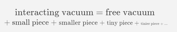
Each of the smaller pieces can be computed through calculating certain scattering processes of the electrons and photons in the free vacuum, and is proportional to increasing powers of $\alpha$.
(In reality the series is a bit more complicated: if you would like a technical account on how it works in the context of the g-factor, then see my Physics.SE answer here).
The process of actually calculating these small pieces relies on the techniques of quantum field theory, and is ostensibly a bunch of extremely complicated and often divergent integrals that one has to make sense of. Feynman found a way to illustrate these integrals in a simple manner, through his diagrams (though they’re still very difficult to understand and compute!).
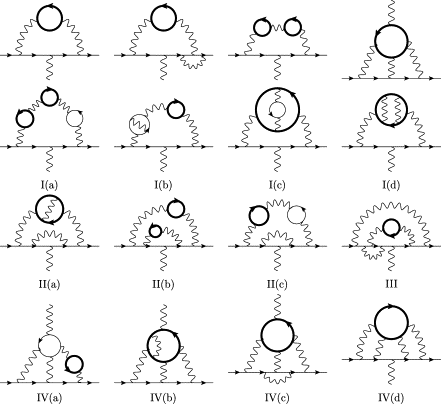
If you look at the previous diagram, you’ll notice that the only lines are an arrow going in, an arrow going out, and a squiggly line. The former two represent the electron, and the last is a photon. This represents the intuitive notion that the magnetic moment can be calculated by looking at what happens to an electron in an external electromagnetic field (specifically, the magnetic part).
The diagram series
These Feynman diagrams can be grouped according to the number of vertices that they have - and the sum of all the diagrams in one group is, roughly, a function of $\left(\frac\alpha\pi\right)^{v-1}$ where $v$ is the number of vertices. So with increasing vertices, the diagrams contribute a smaller amount, and adding up all of these gives us the precise value. Unfortunately, even at 5 vertices there are some 10,000 different diagrams, but computers have managed to do this explicitly.
Schwinger, Feynman and Tomonaga all discovered the first order result independently, and presented their findings at the APS meeting in January 1948:
$$
g=2+2F_2(0)
\\F_2(0)=\frac{\alpha}{2\pi}
\\g=2+\frac\alpha\pi+... = 2.00232
$$
This was an improvement over Dirac’s result of $g=2$ by 3 significant figures, and a triumphant confirmation of the success of QFT. Indeed, the value $\frac{\alpha}{2\pi}$ is engraved on Schwinger’s gravestone.
One quibble: naturally, one would imagine that the other fundamental fields in the Standard Model (say, the gluon field) might also modify the electon g-factor. As it turns out, these contributions are negligible due to the small electron mass - but the mystical muon provides an avenue to incorporate these corrections, and brings with it the alluring possibility of discovering new physics. Stay tuned for more.