
Welcome. In this post, I’ll be describing my implementation of the collider and rigidbody classes. If these terms are unfamiliar, I recommend you take a quick look at my previous post, where I provide an overview of the various components of a physics engine. To summarise: a rigidbody stores the physics properties of the GameObject, while the collider stores its shape and material properties. Although (or perhaps because) these two classes form the core of any physics engine, they are comparatively straightforward and generic.
All of the code is written in Python, and is taken from my physics engine implementation on Github. In turn, these files were essentially transcribed from my original project in Rust, which is still incomplete (I ended up sticking with the Python rendition).
rigidbody.py
class Rigidbody():
    def __init__(self, mass, inertia, position, angle=0):
        self.inv_m = 0 if mass == 0 else 1. / mass
        self.inv_i = 0 if inertia == 0 else 1. / inertia

        self.p = position
        self.v = np.zeros(2)
        self.f = np.zeros(2)

        self.a = angle
        self.w = 0.
        self.t = 0.

        self.R = np.zeros((2, 2))
        self.updateR()

        self.awake = True

    def updateR(self):
        c, s = np.cos(self.a), np.sin(self.a)
        self.R[0, 0] = self.R[1, 1] = c
        self.R[1, 0] = s
        self.R[0, 1] = -s

    def add_force(self, force, at):
        self.f += force
        self.t += np.cross(at - self.p, force)

    def add_impulse(self, impulse, at):
        self.v += self.inv_m * impulse
        self.w += self.inv_i * np.cross(at - self.p, impulse)

    def update(self, dt):
        self.v += self.f * self.inv_m * dt
        self.p += self.v * dt
        self.f = np.zeros(2)

        self.w += self.t * self.inv_i * dt
        self.a += self.w * dt
        self.t = 0.

        self.updateR()

    def l2g(self, v, vec=False):
        return v @ self.R if vec else v @ self.R + self.p

    def g2l(self, v, vec=False):
        return v @ self.R.T if vec else (v - self.p) @ self.R.T
Some comments:
-
It’s easier to directly store the inverse of mass or inertia, since we then have to avoid computing $1/ m$ at each timestep. Divisions are expensive!
- In 2D, all angular variables are scalars. In 3D, angular variables are also 3D, but this is more a coincidence than anything; this relation does not hold in any other dimension
-
We store both the scalar angle as well as the orientation matrix \(\begin{pmatrix}\cos\theta&\sin\theta\\-\sin\theta&\cos\theta\end{pmatrix}\) which is much more useful to convert vectors and points from global to local frame and vice versa. We must make the distinction between vectors and points here, since vectors are only defined by the difference between two points and so need not be translated between frames.
-
Methods are provided to update both force and impulses. This is foreshadowing: for reasons of stability and accuracy, the physics engine will work directly at the level of impulses while resolving constraints. These also add in torque and angular velocity respectively, which are constructed through the cross product: $\tau_\text{2D}=\lVert\vec r\times\vec F\rVert$.
-
The velocity and position (and their angular counterparts) are then updated by the discrete versions of the equations $\Delta \vec v=\int\mathrm dt\ \vec a\Rightarrow\Delta \vec v=m^{-1}\vec F\Delta t$. $\Delta t$ is determined by the frame rate and supplied by the engine in order to keep the updates smooth. Importantly, velocity is updated before the position, so the position update employs the new velocity. This is the Semi-implicit Euler method of integration, and surprisingly yields a lower error than if we were to integrate them in the reverse order.
- Inertia is much easier to implement in 2D than in 3D, where inertia becomes a whole tensor and has to be updated based on the orientation matrix (which, incidentally, requires renormalisation, often using quaternions)
collider.py
class AABB():
    def __init__(self, min_, max_):
        self.min, self.max = min_, max_

    def intersects(self, other):
        return ((self.min <= other.max) & (self.max >= other.min)).all()

    def glVerts(self):
        return (self.min[0], self.min[1], self.max[0], self.min[1],
             self.max[0], self.min[1], self.max[0], self.max[1],
             self.max[0], self.max[1], self.min[0], self.max[1],
             self.min[0], self.max[1], self.min[0], self.min[1])

class Collider():
    def __init__(self, verts, restitution=1.0, friction=.8, density=1.0, offset=np.zeros(2)):
        self.density = density
        self.area = 0
        self.centroid = np.zeros(2)

        vverts = np.zeros((verts.shape[0] + 1, verts.shape[1]))
        vverts[:-1], vverts[-1] = verts, verts[0]

        for i in range(vverts.shape[0] - 1):
            a = vverts[i, 0] * vverts[i + 1, 1] - vverts[i + 1, 0] * vverts[i, 1]
            self.area += a
            self.centroid += a * (vverts[i] + vverts[i + 1])

        self.area *= 0.5
        self.centroid /= 6 * self.area
        self.verts = verts - self.centroid + offset
        self.res = restitution
        self.mu = friction

    def edges(self):
        edges = np.zeros_like(self.verts)
        edges[:-1] = self.verts[1:] - self.verts[:-1]
        edges[-1] = self.verts[0] - self.verts[-1]
        return edges

    def aabb(self):
        return AABB(np.min(self.verts, axis=0), np.max(self.verts, axis=0))

    @staticmethod
    def regular_polygon(n, size):
        verts = np.exp(np.arange(n) * np.pi * 2j / n) * size
        return Collider(verts.view('(2,)float'))

    @staticmethod
    def random_polygon(n, size):
        angles = np.cumsum(np.random.rand(n))
        angles = angles / np.max(angles)
        verts = np.exp(angles * np.pi * 2j) * size
        return Collider(verts.view('(2,)float'))
-
First, the Collider class: it stores an ordered set of vertices and material properties such as the friction and restitution (“bounciness”). Using the shoelace formula and its derivatives, we can compute the centroid and area of the polygon, the latter of which can be multiplied with density to obtain the mass of the collider. However, since we envision objects with multiple colliders associated to them, an offset can also be supplied, which translates the centroid of the collider away from the true centre of the composite object.
-
There are also straightforward methods for obtaining the edges of the collider and regular and random convex polygons. The latter algorithm is neat: random angles between $0$ and $2\pi$ are generated and then the points on a circle corresponding to these angles are sewn up.
-
Now for the AABB (axis-aligned bounding box) class. This is simply a non-rotated rectangle which encloses the polygon perfectly, and is specified by its bottom-left and top-right corner positions. This solely exists to improve collision detection speeds: rather than immediately jumping into an expensive collision detection routine for each pair of bodies, we can instead discard a sizeable portion of the pairs if their AABBs do not intersect (the intersection test for AABBs is extremely fast). After isolating those pairs which actually stand a chance of intersecting, we perform the full-fledged SAT-GJK routine to identify the true positives. Some people use oriented bounding boxes, where the bounding rectangle can be rotated. This leads to tighter fitting boxes and hence better pair pruning, at the expense of a more involved and time-consuming computation and intersection test.
What is a Physics Engine?
It’s simply a framework that allows you to simulate the effects of physics on objects. The physics engine on its own merely performs computations on vectors, so it is typically accompanied by a graphics or render engine, with which it runs in tandem. The level of realism achieved by the physics engine varies greatly depending on the requirements, with real-time game physics engines sacrificing pinpoint accuracy to preserve FPS and realistic fluid simulations for research doing precisely the opposite. Rendered physics in movies, for instance, lies somewhere in between.
A major component of physics engines is the so-calles “rigid bodies”, which are non-deformable objects with a definite shape. Computationally this is nice because at each instant, the body can be specified by a precomputed fixed shape and a single position and angle, which is then passed onto the renderer to display the object on screen. Although we live in a world with continuous time, physics engines discretise it, but since the laws of motion are formulated using calculus, we must employ an “integrator” to yield physically realistic results using a discrete approximation.
Other aspects that a physics engine has to tackle is collisions between shapes - detecting and resolving them - as well as constraints such as hinges and ball-and-socket joints. On the surface these appear to be completely different problems, but a constraint-based physics engine actually implements these in exactly same manner, and I will have a great deal to say about this in later blog posts.
How did I make it?
I was initially drawn to making game physics engines when I was in around 8th grade, before I even knew much physics. But I had just learned integral calculus, so it seemed like a reasonably “extended” project that I could attempt with my newfound skills. My language of choice was Java (with Swing), and I ended up making a decent, simple physics engine - you could add circles of different sizes, masses and restitutions and make them bounce off each other and walls.
A couple of years later I decided to revisit this and completely revamp it, using the more powerful constraint-based approach, and allowing for more complex shapes, rotations, friction, and constraints.
Instead of continuing with Java and its annoying absence of operator overloading, I opted for Python, which provides the incredibly powerful NumPy library for linear algebra in computational science. Bear in mind that I was just cooling off from a couple months’ obsession with machine learning, so I was adept at computational linear algebra even before starting.
NumPy for the physics part was inevitable, but I had a few options for the animation toolset. Eventually I settled with the Pyglet package, which was reasonably concise since it used OpenGL-like syntax.
I’ll give an overview of the various components of my physics engine here, and you can find an in-depth explanation in the links provided.
-
The core rigidbody is very straightforward - the basic features are attributes for mass, position, velocity and acceleration vectors (and their angular counterparts). You provide a callback to update these values at a timestep, using the accumulated force, velocity, etc. to update the velocity, position, etc. The final element is a function to convert from the rigidbody frame to the global frame and vice versa.
-
The collider (I used Unity’s terminology) encodes the actual shape of the object in question, simply specified by a list of coordinates in global frame, from which the centre of mass is computed by the shoelace formula. It also stores restitution and friction, since multiple colliders can be assigned to a single rigidbody to create a composite shape. The main method here is to return the axis-aligned bounding box, a non-rotated bounding rectangle which speeds up detection of polygon intersection by providing a quick way to discard true negatives.
-
The GameObject is the container of one or more colliders, and a rigidbody for centre of mass motion. It provides a static function for determining whether two GameObjects are intersecting (a position update at a timestep may push one body slightly into another), and returns one or more “contact manifolds” containing details of such an intersection, if present. Collision detection for arbitrary polygons is rather difficult - here I restrict to convex polygons only, and I employ the SAT algorithm, which is quite tricky to get right.
-
The Constraint class is an abstract parent class of the various types of constraints - one is of course the contact constraint, and others include the fixed distance constraint and the prismatic joint. These are defined to constrain two GameObjects, and can cache and return a “Jacobian” which characterises the violation of the constraint at the current time step
-
The physics engine itself controls the timestepping and intervals, carefully inserting extra frames to regulate smoothness, and passing the $\Delta t$ parameter which controls the integrator mentioned above. At each time step, it also solves the constraints and applies external forces to update the bodies.
-
The graphics engine runs at its own pace, rendering the colliders of all GameObjects in the scene
Conceptually, these elements are quite simply, but implementing an engine that is both accurate and fast is quite an optimisation challenge, so there are several complicated features that can go into making such an engine.
String Dualities
The five superstring theories that we’ve been constructing are all beautiful, but the fact that there are five of them in the first place is somewhat mysterious. This puzzled string theorists long past the first superstring revolution, but the second superstring revolution brought with it a radical idea - what if all these ostensibly different theories were really related, and so incarnations of a deeper, more fundamental theory?
Let us motivate the nature of these relations with the bosonic string. Recall from last time’s discussion that “string compactification” does not imply topologically manipulating an initial spacetime, but rather positing the exact structure of spacetime right from the get go. Since bosonic string theory operates peacefully in 26 dimensions, choose a spacetime which is a “product manifold” of 24+1D Minkowski space and a 1D circle of some radius $R$. In ordinary terms, the 26th dimension is circular (as a consequence, you can travel in the same direction and come back to your starting point) while the remaining dimensions are flat. Note that despite being circular, this dimension is not necessarily “curled up” in the sense of being comparatively microscopic - this is determined by the radius $R$ which for now remains a free parameter. Now closed strings can wrap around this circular dimension multiple times, akin to a rubber band wrapped around a tube. If a string winds $N$ times around a circle, then clearly it must have a length of at least $2\pi RN$.
The idea of introducing one circular dimension is surprisingly ancient. First proposed by Kaluza in 1921 (general relativity was just beginning to gain traction while the Schrödinger equation had not even been formulated yet!) and refined by Klein, this theory unified gravitation and electromagnetism by hypothesizing a 5D spacetime with the 5th dimension forming a circle. This operated on a purely classical footing, and interestingly, “motion in the fifth dimension” is roughly identified with the charge of the particle. It additionally predicted a dynamical scalar fields, which could serve as a parameter for the expansion of spacetime, or even a coupling between gravity and electromagnetism, depending on the model. This was an early demonstration of how compact dimensions, even at a classical level, can yield exciting new physics.
A main feature of a compact dimension is that momentum along that dimension is quantised: it comes in multiples of $1/R$. This is in contrast to an infinite dimension, where momentum is continuous (this is also clear by taking the $R\to\infty$ limit above - in this limit, a circular dimension unrolls). For the reason, hark back to the quantized momentum levels of a particle in a periodic box - or, if unfamiliar, appeal to the following heuristic description: a particle is described by a wavefunction; with periodic boundary conditions, the particle must form standing waves whose wavelength is a multiple of the box width (other waveforms are suppressed by destructive interference), so wavelength is quantized. But quantum mechanical momentum is inversely proportional to wavelength, so it too is quantized! The $p\propto1/R$ dependence is manifest here - we write that $p=K/R$.
Ordinarily the mass of a particular string state depends on the total number of left-moving excitations and right-moving excitations. However, now that we have a compact dimension, the winding number $N$ and the so-called “Kaluza-Klein excitation number” $K$. The winding number contributes a term $\left(\frac{NR}{\alpha’}\right)^2$ where $\alpha$ is roughly the string tension, while the KK-momentum adds a $\frac KR$ term. Clearly both $N$ and $K$ can be any non-negative integer, depending on the configuration of the string in question.
Here’s the surprising part. What if we had the audacity to switch $N$ and $K$? This would be extremely unexciting were it not for the fact that, upon switching $R$ with $\alpha’/R$ simultaneously, all the formulas remain the same! In other words, compactifying string theory on a circle of radius $R$ yields the same physics as if we were to compactify on a circle of radius $\alpha’/R$. The only difference is that winding numbers and KK momentum number in one theory correspond to KK momentum and winding number in the other - but since both of these could be any non-negative integer anyway, there is no physical difference! Importantly, this $N\Leftrightarrow K, R\Leftrightarrow\alpha’/R$ transform can be equivalently expressed as vertically mirroring the right-moving, but not left-moving, excitations of the string.
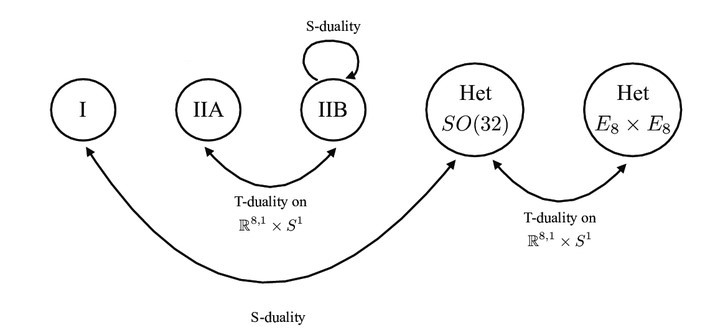
Since this forms an equivalence between two rather different looking theories: one string theory (model) whose radius in the 26th dimension is, say, $0.001\text{ m}$, and another whose radius is $1,!000\text{ m}$. This is our first example of a string duality, known as T-duality. This duality will manifest in a deeper form in superstring theory, as we shall see. T-duality also has interesting effects on D-branes, depending on their orientation, but I will not discuss those here.
Let’s start with Type IIA theory. It is more helpful to apply the second incarnation of T-duality: vertically flipping the right-moving modes. Since this is a superstring theory, we only have 10 dimensions to play with, so let’s compactify the 10th dimension on a circle. The right-moving component of the bosonic coordinate is flipped, which also interchanges the winding number and KK-momentum and converts the radius of compactification from $R$ to $\alpha’/R$, as we have seen. As for the partner fermionic coordinate, we would intuitively think that supersymmetry on the worldsheet forces its right-moving part to flip in the same way, and indeed it does. It is important to always keep in mind that applying T-duality never changes the physics, only the mathematical form the theory takes.
But we know that relative signs of fermions play a huge role in distinguishing the two Type II string theories. Indeed, flipping the right-moving sector reverses the chirality of the fermions associated to it. Let’s see what happens to Type IIA string theory as a result. By definition, it has fermions of opposite chiralities amongst its left and right movers. T-duality inverts the compactification radius and flips the chirality of the right-moving fermions, so now we have fermions of the same chirality in both sectors. But this is just the definition of Type IIB string theory! Type IIA compactified on a circle of radius $R$ is the exact same theory as Type IIB compactified on a circle of radius $\alpha’/R$ - they should really be thought of as one unified theory! So unlike in the bosonic case where T-duality related a theory to itself, two different superstring theories are united by this duality.
To relentlessly spring another surprise, it turns out that the two heterotic string theories are also related by T-duality! Here, the analysis is much more difficult and geometric, but it is sound. So another link has been forged, and the castles are no longer isolated.
But there is yet another type of duality. A small motivation (which may not actually be very enlightening, but is a fun morsel nonetheless) can be seen if we beam ourselves down to ordinary electromagnetism. In its classical, non-covariant formalism, there are two fields - the electric and the magnetic - permeating throughout space, interacting with charged particles. The evolution of such fields with time is determined by Maxwell’s equations - for instance, the evolution of the electric field is determined by the charge distribution and the rate of change of the magnetic field. If we take the simple cases where no charges or currents exist (the theory may seem trivial, but it still allows for the propagation of electromagnetic waves), then Maxwell’s equations show a surprising symmetry of sorts: if you interchange (roughly) the electric field with the magnetic field, the equations remain the same. As it turns out, an analogue of this relation carries forth to supersymmetric gauge theories and string theory, where it is christened S-duality.
The main way to practically compute quantities in string theory is to “expand the theory in $\alpha’$”. What this means is that we recognise that the string is an extended (not point) object, and this presents computational difficulties, so we initially pretend it is a perfect point particle and layer on stringy corrections on top of this. It is akin to approximating a function by a Taylor expansion in ordinary calculus.
However, there is also another type of expansion that we must factor in: that of string interactions. The strength of interactions is described by the value $g_s$, the string coupling constant. Roughly, a small value of $g_s$ describes a system in which strings interact weakly, and so we can Taylor expand from the free, non-interacting theory as a base point, which itself serves as a good approximattion. However, at high $g_s$, the strings are strongly coupled, and the analysis becomes very complicated since strings are continuously interacting, and it becomes difficult to entangle them, so to speak. Coupling constants are of course ubiquitous in quantum field theory as well. In quantum electrodynamics, the coupling constant is proportional to the square of the electron’s charge, with some more fundamental constants added in too. This coupling constant is weak, at around $1/137$ (dimensionless), which means that approximating the theory as non-interacting, then adding corrections for the interactions weighted by powers of the coupling constant is valid, and indeed this is how computations are performed. However, quantum chromodynamics has a coupling constant which is around $1$, and so this series method breaks down as the additional terms in the series all have the same size, so we won’t ever be able to get a good approximation by truncating this sum at some point. Consequently, non-perturbative methods which do not rely on performing this sum are utilised, such as lattice QCD, in which spacetime is discretised and the lattice spacing is then taken to zero in order to recover continuous spacetime (this is a huge subfield of its own). String theory differs from the above in that the value of this coupling constant is determined dynamically by the value of a particular scalar field known as the dilaton: $g_s =\exp\langle\Phi\rangle$, or in words, the strength of the string interaction is determined by the average value of the dilaton field in a vacuum. Like all quantum fields, the dilaton is subject to quantum fluctuations, but in this definition we average over all such fluctuations.
Returning to string theoretic apprxomations, we may additionally opt to neglect string states with high mass, as they are very difficult to produce and so do not contribute substantially to observable quantities, at least at low energies below their production level. In the extreme limit, we can disregard all states with mass and simply consider the massless fields, while taking $\alpha’\to 0$. This creates the low-energy effective action of string theory, which is seen to be supergravity (SUGRA) in 10D, as I have mentioned before. However, the validity of SUGRA only extends as far as low to intermediate energies - it is seen to break down at high energies, which signals that there must be a more complete thoery which subsumes it. Indeed, the various string theories form these UV-completions of the different supergravities.
SUGRA tends to be easier to manipulate, and we can identify tools and hints of physics that goes on in string theory, even if we cannot directly extrapolate results. In particular, consider the low-energy effective actions of type I and $\mathrm{SO}(32)$ heterotic theory. Their mathematical forms are extremely similar, as they are related via negating the dilaton field ($\Phi\Leftrightarrow-\Phi$) and conformally scaling the metric (the metric is the field which determines the spacetime geometry, including distances, angles and of course gravitational effects). This conformal scaling preserves the angles of the spacetime geometry but alters distances non-uniformly - this merely suggests that the two different spacetimes are mapped to each other. Once again, since string theory allows any spacetime to serve as a background (provided of course that they are consistent with Einstein’s equations of general relativity, which the conformal rescaling preserves), this is a perfect symmetry of the two theories.
The negation of the dilaton is extremely important. If we pretend that this relation holds not only for supergravity, but also for the entire string theory, then since the string coupling constant is determined by $\exp\langle\Phi\rangle$, we see that a coupling of $g_s$ in type I would correspond to a coupling of $1/g_s$ in $\mathrm{SO}(32)$ heterotic. In other words, S-duality is suggesting that strongly coupled interactions in one theory can be described by weakly coupled interactions in the other theory. As a result, they should once again be regarded as two facets of the same underlying theory.
From this we can conclude with certainty that type I string theory and $\mathrm{SO}(32)$ heterotic theory are equivalent when probed at low energies. But does this duality extend to the full string theory at all energies? This is diffcult to check directly, since by definition probing the effects of strongly coupled string interactions (to verify the duality) is intractable. However, there are certain tests that rely on non-perturbative effects, for example, matching the tension of D-branes on either side of the duality. So far, S-duality has passed all tightly-constraining theoretical checks, and is regarded as an exact duality. However, we do not have a 100% rigorous proof for this, unlike T-duality which is very easy to verify. This method of conducting theoretical consistency checks to verify S-duality is a general feature of such dualities in supersymmetric gauge theories.
The final manifestation of duality in string theory is once again an S-duality, but this time it concerns type IIB string theory. The spectrum of this theory includes within it a massless dilaton $\phi$ (every string theory does, in the bosonic sector) but also a massless scalar field $C_0$ from the fermionic sector, known as an RR zero-form gauge field. This feature is unique to type IIB, and means that it has a symmetry that mixes the two fields into each other. Interestingly, due to stringy effects, the symmetry is not continuous (like a rotation), but rather discrete (like translation along a lattice). One such discrete symmetry transformation, when evaluated at vanishing $C_0$, once again flips the sign of the dilaton, which as we have seen corresponds to sending the coupling constant $g_s$ to $1/g_s$. So S-duality implies that Type IIB string theory is self-dual, and strongly coupled effects can be described by effects at weak interactions, and vice versa.
This concludes the beautiful web of dualities that connect and unify all the superstring theories. They are mathematically breathtaking, and will be studied for years to come.
But I leave you on one note. All 5 string theories are now connected. Can we build one single fundamental, underlying description of all of them together? Would such a theory be consistent? What would it look like? How would it reduce to the existing string theories? Tell us more!
Edward Witten in 1995 told us the answer. The fundamental theory, uniting all of string theory together, operates in 11 dimensions. They call this beast M-theory.
But it is not a theory of strings…
In the previous post, we looked at the construction of superstring theory, but to our surprise, found two slightly different methods of constructing it! Now we will explore what the difference between the two is, and whether they are consistent. Be prepared for a couple of surprises along the way.
Superstring theories!?
But first, a detour into spin. To this date, spin remains the most misleading piece of terminology since nothing is actually spinning in a fundamental particle! Rather, it consitutes an intrinsic angular momentum of the particle, and is not ad hoc, but a direct consequence of unifying quantum mechanics with special relativity. Like any vector, the spin of a particle can point in a particular direction and, for example, the relative direction between the spin and an external magnetic field determines the strength of the interaction and hence the magnitude of the force experienced by the particle.
For massless particles, we can define a related concept called helicity. A massless particle is left-handed if its spin and momentum are antiparallel, and right-handed if they are parallel. If it seems peculiar to ascribe momentum to a massless particle, recall that $p=\frac Ec$ according to special relativity. The idea of helicity coincides with a related but distinct property called chirality for massless particles, which will be of interest here.
Now theorists have been continually interested in symmetries of nature. In particular, there were three eminent discrete symmetries that were regarded as sacrosanct: charge (C) symmetry, parity (P) symmetry and time-reversal (T) symmetry. Roughly, C-symmetry flips all the internal quantum numbers of every particle (e.g. electrical charge), P-symmetry replaces left with right, and T-symmetry reverses the direction of time. Electromagnetism, the strong force and gravity all preserve each of these independently. Unfortunately, the pesky weak force violated both C-symmetry and P-symmetry. It was subsequently hoped that CP-symmetry (flipping charges and direction simultaneously) would be respected, but further experiments involving decays of neutral kaons discredited this, and indirectly destroyed T-symmetry as well. The only discrete symmetry which the Standard Model assumes to hold exactly is CPT-symmetry, a combination of all three inversions simultaneously. Theories like the Standard Model which do not respect CP-symmetry are said to be chiral, and any master-theory that subsumes it must provide a mechanism to generate this asymmetry.
Back to strings! Once we perform a GSO projection on the left-movers, we can choose to perform the same projection, or the other projection on the right-movers. Naturally, choosing identical projections results in the massless fermions in the theory having the same chirality, resulting in Type IIB string theory, while choosing opposite projections makes the theory non-chiral, forming Type IIA string theory. The “II” in both cases refers to the $\mathcal N=2$ supersymmetry that they display, with each boson having two partner fermions and vice versa. To ensure that all the states are physical, the dimension of spacetime is forced to be 10 - much less than the 26 required for bosonic string theory! The fact that type IIB string theory is chiral makes it very useful for string phenomenology and realistic model building.
This should be the end of the story, but string theory continues to yield new surprises. The type IIB theory has a worldsheet parity symmetry, where the left-moving modes and right-moving modes are exchanged. Since both sectors have the same chirality, this renders the theory invariant. This does not mean that each state is parity invariant: considering the function ${1, 2, 3, 4}\to{1, 3, 2, 4}$, the set (the “theory”) remains invariant, but only the subset ${1, 4}$ (the “parity-invariant states”) are mapped to themselves. Naturally the situation is a little more complicated (different parts of each sector can “decompose” into variant and invariant pieces), but the general idea persists. What if were to “gauge” this symmetry, which would amount to projecting type IIB string theory down to only those components which were left-right symmetric?
First success - the graviton is symmetric, so it survives the projection. We still have a theory of quantum gravity! The massless gravitino also survives, forcing spacetime supersymmetry for consistency. We breathe a sigh of relief when we see that the number of degrees of freedom match in the fermionic and bosonic sectors: we have constructed a new, consistent string theory. This has some interesting features, as we shall see.
Firstly, the parity projection destroys half the amount of supersymmetry, so there is only one superpartner for each particle. This is $\mathcal N=1$ SUSY, so we have obtained Type I string theory. Another curious aspect is the presence of open strings in the theory. Imagine a -multi-coloured loop (a “closed string”) which is left-right symmetric. The projection operator “squashes” this circle vertically into a symmetric string with disjoint ends (the open string!). The once oriented fundamental string now yields both unoriented closed strings and unoriented open strings in type I string theory.
Now the ends of these strings can have different internal charges associated with them. Determining how these charges should transform under the parity operator is initially mystifying, but experience tells us to search for and impose consistency requirements. This time we must explore the low-energy behaviour of string theory. Eliding all the mathematical details, string theory at low energies looks like a supersymmetric theory of gravity with the same value of $\mathcal N$, in the same number of spacetime dimensions. This is akin to how molecular interactions are constantly fizzling inside water, but we sweep over these microscopic details while building an accurate description of the “big picture”, as in fluid dynamics. In the case of string theory this correspondence is arguably stronger since the relation holds on purely mathematical grounds rather than having to appeal to observation. As it turns out, $\mathcal N=1$ supergravity in 10D is inconsistent on its own due to so-called “anomalies”.
The only way to remedy this to fuse supergravity with a particular type of Yang-Mills theory, which is an analogue of electromagnetism in which charges can interact with themselves - for instance, in QCD, gluons are self-interacting. Such a Yang-Mills theory is uniquely specified by a choice of dimension and “gauge group”, a deep mathematical object whose mathematical beauty I cannot overstate, but also cannot explain due to a lack of space here - one may regard them merely as “data” here. The only gauge groups which work are $\mathrm{SO}(32)$ and $E_8\times E_8$, but the latter is not compatible with the open type I string. So the gauge group of the low-energy effective theory, and by extension the open string, is mathematically and uniquely determined to be $\mathrm{SO}(32)$, and this in turn fixes the transformation properties of the internal charges on the ends of the string.
The final (and my personal favourite) feature is the existence of D-branes. Briefly, a D-brane is a hypersurface (a high-dimensional object) on which the end of an open string can lie. If the ends of the string are unconstrained, one obtains a D9-brane which fills all of spacetime (the number after the “D” indicated the number of spatial dimensions only. So a D9-brane for instance has 9 spatial dimensions and one time dimension, as does spacetime). In type I superstring theory, there also exist D1 and D5 branes. The idea initially seems rather unhelpful, and possibly downright useless. However, Polchinski in 1995 discovered that the branes themselves carry charges, and so, to supplement the fundamental string, should be regarded as dynamical objects in their own right! Furthermore, they are adored by phenomenologists because branes intersecting along different dimensions give rise to lively, interacting gauge theories on their surface, and specific brane constructions and backgrounds can be used to create realistic models of the universe!
That concludes this whirlwind tour of string theory. Haha, no, there’s more. It sounds ridiculous, but we can use the bosonic string construction for the left-movers, and the superstring construction on the right-movers in order to create a new string theory! This should trigger instant revulsion - isn’t there a dimensional mismatch between the two sides? Naïvely yes, but we can introduce a 16-dimensional toroid with a particular gauge symmetry to offset this. We obtain another consistent $\mathcal N=1$ string theory, and we know from above that we should use the $\mathrm{SO}(32)$ gauge group with this toroid. We have constructed $\mathrm{SO}(32)$ heterotic string theory! But we’re still not done. This time, the $E_8\times E_8$ group is also compatible, so we can create (or rather, discover) the $E_8\times E_8$ string theory as well. This beast is well suited for model building, since a unified fundamental force embeds very nicely within this gauge group.
And that, ladies and gentlemen, is how the five superstring theories (and their little brother, the bosonic string) were discovered. As an afterword, I would like to ease your likely persistent discomfort at how string theory could ever explain the universe. After all, we see only 4 dimensions. This is solved rather straightforwardly through the process of compactification.
Now string theory has no preference to the geometry of spacetime. As such, we can posit that the 10D background is really a product of ordinary 4D macroscopic spacetime, and a curled-up 6D surface which at ordinary energies, yields microscopic directions that cannot be probed. If this also sounds ad hoc, it is imperative to understand the fundamental nature of string theory: it is not a “theory” in the conventional sense. It is a framework, much like quantum field theory. Just as QFT serves a language in which the Standard Model (a true theory) can be written, string theory can be used to construct models with whatever features we desire.
As mentioned in the previous blog post, supersymmetry would solve a lot of problems in the Standard Model and cosmology, and it is generally expected to exist at high energies on empirical grounds. So we would like this string compactification to preserve $\mathcal N=1$ SUSY, the simplest, most constraining form of supersymmetry. A beautiful result here is that the geometry of this 6D “internal” manifold determines the amount of supersymmetry preserved, in addition to other predictive features like the number of generations of fundamental particles (the Standard Model has three generations). If, for example, we start with $\mathcal N=2$ type IIB string theory, compactifying on a Calabi-Yau manifold creates a $\mathcal N=1$ field theory. As I also mentioned previously, we can fiddle around with D-brane backgrounds and fluxes to generate models. A key geometrical result is that the number of realistic compactifications is on the order $10^{500}$, a humongous but number. This is just one of the reasons string theory is held in high regard by many people.
However, if this five-fold disjunction of string theories smacks to you of inelegance, you are not alone. This puzzled superstrings long past the superstring revolution, but it led to the most beautiful result in superstring theory. Stick around to find out.